Molecular dynamics simulations of bulk water

In this example, we show how to perform molecular dynamics of bulk water using the popular interatomic TIP3P potential (W. L. Jorgensen et. al.) and LAMMPS.

import numpy as np
%matplotlib inline
import matplotlib.pylab as plt
from pyiron import Project
import ase.units as units
import pandas

pr = Project("tip3p_water")

Creating the initial structure

We will setup a cubic simulation box consisting of 27 water molecules density density is 1 g/cm\(^3\). The target density is achieved by determining the required size of the simulation cell and repeating it in all three spatial dimensions

density = 1.0e-24  # g/A^3
n_mols = 27
mol_mass_water = 18.015 # g/mol

# Determining the supercell size size
mass = mol_mass_water * n_mols / units.mol  # g
vol_h2o = mass / density # in A^3
a = vol_h2o ** (1./3.) # A

# Constructing the unitcell
n = int(round(n_mols ** (1. / 3.)))

dx = 0.7
r_O = [0, 0, 0]
r_H1 = [dx, dx, 0]
r_H2 = [-dx, dx, 0]
unit_cell = (a / n) * np.eye(3)
water = pr.create_atoms(elements=['H', 'H', 'O'],
                        positions=[r_H1, r_H2, r_O],
                        cell=unit_cell, pbc=True)
water.set_repeat([n, n, n])
water.plot3d()

water.get_chemical_formula()

'H54O27'

Equilibrate water structure

The initial water structure is obviously a poor starting point and requires equilibration (Due to the highly artificial structure a MD simulation with a standard time step of 1fs shows poor convergence). Molecular dynamics using a time step that is two orders of magnitude smaller allows us to generate an equilibrated water structure. We use the NVT ensemble for this calculation:

water_potential = pandas.DataFrame({
    'Name': ['H2O_tip3p'],
    'Filename': [[]],
    'Model': ["TIP3P"],
    'Species': [['H', 'O']],
    'Config': [['# @potential_species H_O ### species in potential\n', '# W.L. Jorgensen et.al., The Journal of Chemical Physics 79, 926 (1983); https://doi.org/10.1063/1.445869\n', '#\n', '\n', 'units real\n', 'dimension 3\n', 'atom_style full\n', '\n', '# create groups ###\n', 'group O type 2\n', 'group H type 1\n', '\n', '## set charges - beside manually ###\n', 'set group O charge -0.830\n', 'set group H charge 0.415\n', '\n', '### TIP3P Potential Parameters ###\n', 'pair_style lj/cut/coul/long 10.0\n', 'pair_coeff * * 0.0 0.0 \n', 'pair_coeff 2 2 0.102 3.188 \n', 'bond_style harmonic\n', 'bond_coeff 1 450 0.9572\n', 'angle_style harmonic\n', 'angle_coeff 1 55 104.52\n', 'kspace_style pppm 1.0e-5\n', '\n']]
})

job_name = "water_slow"
ham = pr.create_job("Lammps", job_name)
ham.structure = water
ham.potential = water_potential

/srv/conda/envs/notebook/lib/python3.7/site-packages/pyiron/lammps/base.py:170: UserWarning: WARNING: Non-'metal' units are not fully supported. Your calculation should run OK, but results may not be saved in pyiron units.
  "WARNING: Non-'metal' units are not fully supported. Your calculation should run OK, but "

ham.calc_md(temperature=300,
            n_ionic_steps=1e4,
            time_step=0.01)
ham.run()

The job water_slow was saved and received the ID: 1

view = ham.animate_structure()
view

Full equilibration

At the end of this simulation, we have obtained a structure that approximately resembles water. Now we increase the time step to get a reasonably equilibrated structure

# Get the final structure from the previous simulation
struct = ham.get_structure(iteration_step=-1)
job_name = "water_fast"
ham_eq = pr.create_job("Lammps", job_name)
ham_eq.structure = struct
ham_eq.potential = water_potential
ham_eq.calc_md(temperature=300,
               n_ionic_steps=1e4,
               n_print=10,
               time_step=1)
ham_eq.run()

The job water_fast was saved and received the ID: 2

view = ham_eq.animate_structure()
view

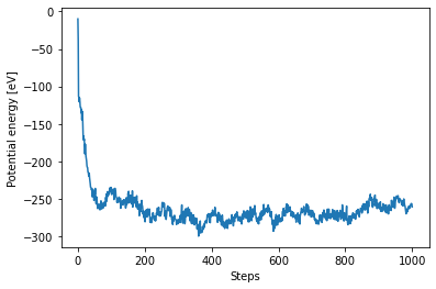
We can now plot the trajectories

plt.plot(ham_eq["output/generic/energy_pot"])
plt.xlabel("Steps")
plt.ylabel("Potential energy [eV]");

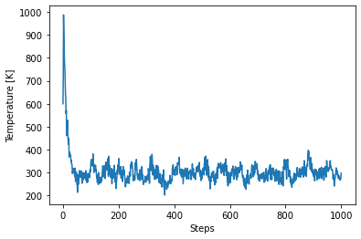
plt.plot(ham_eq["output/generic/temperature"])
plt.xlabel("Steps")
plt.ylabel("Temperature [K]");

Structure analysis

We will now use the get_neighbors() function to determine structural properties from the final structure of the simulation. We take advantage of the fact that the TIP3P water model is a rigid water model which means the nearest neighbors, i.e. the bound H atoms, of each O atom never change. Therefore they need to be indexed only once.

final_struct = ham_eq.get_structure(iteration_step=-1)

# Get the indices based on species
O_indices = final_struct.select_index("O")
H_indices = final_struct.select_index("H")

# Getting only the first two neighbors
neighbors = final_struct.get_neighbors(num_neighbors=2)

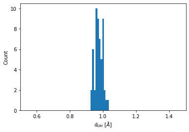
Distribution of the O-H bond length

Every O atom has two H atoms as immediate neighbors. The distribution of this bond length is obtained by:

bins = np.linspace(0.5, 1.5, 100)
plt.hist(neighbors.distances[O_indices].flatten(), bins=bins)
plt.xlim(0.5, 1.5)
plt.xlabel(r"d$_{OH}$ [$\AA$]")
plt.ylabel("Count");

Distribution of the O-O bond lengths

We need to extend the analysis to go beyond nearest neighbors. We do this by using the number of neighbors in a specified cutoff distance

num_neighbors = final_struct.get_numbers_of_neighbors_in_sphere(cutoff_radius=9).max()

neighbors = final_struct.get_neighbors(num_neighbors)

neigh_indices = np.hstack(np.array(neighbors.indices)[O_indices])
neigh_distances = np.hstack(np.array(neighbors.distances)[O_indices])

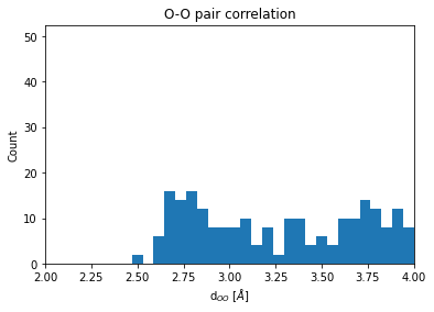
One is often intended in an element specific pair correlation function. To obtain for example, the O-O coordination function, we do the following:

# Getting the neighboring Oxyhen indices
O_neigh_indices  = np.in1d(neigh_indices, O_indices)
O_neigh_distances = neigh_distances[O_neigh_indices]

bins = np.linspace(1, 8, 120)
count = plt.hist(O_neigh_distances, bins=bins)
plt.xlim(2, 4)
plt.title("O-O pair correlation")
plt.xlabel(r"d$_{OO}$ [$\AA$]")
plt.ylabel("Count");

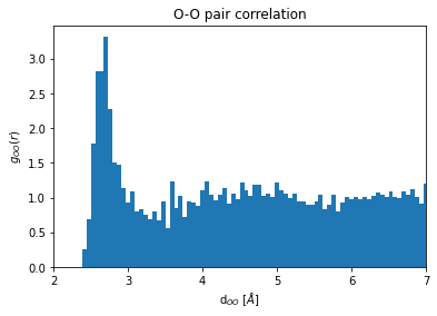
We now extent our analysis to include statistically independent snapshots along the trajectory. This allows to obtain the radial pair distribution function of O-O distances in the NVT ensamble.

traj=ham_eq["output/generic/positions"]
nsteps=len(traj)
stepincrement=int(nsteps/10)
# Start sampling snaphots after some equilibration time; do not double count last step.
snapshots=range(stepincrement,nsteps-stepincrement,stepincrement)

for i in snapshots:
    struct.positions = traj[i]
    neighbors = struct.get_neighbors(num_neighbors)
    neigh_indices = np.hstack(np.array(neighbors.indices)[O_indices])
    neigh_distances = np.hstack(np.array(neighbors.distances)[O_indices])
    O_neigh_indices  = np.in1d(neigh_indices, O_indices)
    #collect all distances in the same array
    O_neigh_distances = np.concatenate((O_neigh_distances,neigh_distances[O_neigh_indices]))

To obtain a radial pair distribution function (\(g(r)\)), one has to normalize by the volume of the surfce increment of the sphere (\(4\pi r^2\Delta r\)) and by the number of species, samples, and the number density.

O_gr=np.histogram(O_neigh_distances,bins=bins)
dr=O_gr[1][1]-O_gr[1][0]
normfac=(n/a)**3*n**3*4*np.pi*dr*(len(snapshots)+1)
# (n/a)**3            number density
# n**3                number of species
# (len(snapshots)+1)  number of samples (we also use final_struct)

plt.bar(O_gr[1][0:-1],O_gr[0]/(normfac*O_gr[1][0:-1]**2),dr)
plt.xlim(2, 7)
plt.title("O-O pair correlation")
plt.xlabel(r"d$_{OO}$ [$\AA$]")
plt.ylabel("$g_{OO}(r)$");